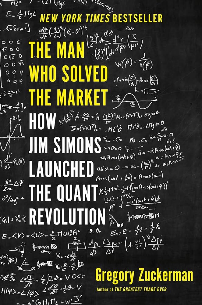
Mathematical Models in Quantitative Finance: An Exploration Inspired by The Man Who Solved the Market
The Man Who Solved the Market by Gregory Zuckerman offers a detailed account of Jim Simons, a renowned mathematician, and his revolutionary hedge fund, Renaissance Technologies. Through meticulous research, Zuckerman sheds light on how Simons transformed the financial world with his unique approach, creating one of the most successful hedge funds in history. This book isn't merely about finance; it delves into the intersection of mathematics, data science, and the sometimes impenetrable world of hedge funds. Here's an analysis of the book's key themes, insights, and contributions to the understanding of modern finance.
Zuckerman does not delve deeply into the specific mathematical equations or algorithms used by Jim Simons and his team at Renaissance Technologies due to the proprietary and secretive nature of their methods. However, the book does hint at the types of mathematical approaches and concepts that Renaissance might have employed. Below are some generalized examples of equations and mathematical techniques typically associated with quantitative finance and algorithmic trading—fields in which Renaissance Technologies excelled.
1. Statistical Arbitrage Models
Statistical arbitrage relies heavily on mean reversion strategies. One common equation used in this context is the Z-Score, which measures how far away a data point is from the mean. The Z-score can be used to determine whether an asset is overbought or oversold relative to its historical average.
The Z-score formula is:
Where:
Z is the Z-score.
X is the current value of the asset.
μ is the mean (average) value of the asset.
σ is the standard deviation of the asset's values.
Traders might use this concept to identify pairs of assets that have historically moved together. When their Z-score diverges significantly, they might anticipate a reversion to the mean, initiating trades accordingly.
2. Moving Averages for Trend Analysis
One common tool in quantitative finance is the Moving Average (MA), which is used to smooth out price data and identify trends over time. A strategy might involve comparing the short-term moving average with a long-term moving average to signal potential buying or selling points.
The formula for a simple moving average is:
Where:
MA is the moving average.
n is the number of periods.
Pi is the price of the asset at each period i.
For instance, if a short-term 50-day MA crosses above a long-term 200-day MA, it might signal a buying opportunity ("Golden Cross"), and a short-term MA crossing below a long-term MA might indicate a selling opportunity ("Death Cross").
3. Linear Regression for Predictive Models
Linear regression can be used to predict the price movement of an asset based on historical data. In finance, a simple form of a linear regression might be:
Where:
y is the dependent variable (e.g., asset price).
x is the independent variable (e.g., time or another asset’s price).
β0 is the intercept.
β1 is the slope (which indicates how much y changes for a unit change in x).
ϵ is the error term.
Quantitative funds like Renaissance often use multivariate regression (with multiple predictors) to predict asset prices or find correlations between different assets.
4. Logistic Regression for Probability Estimation
Logistic regression is often employed when the goal is to predict a binary outcome, such as whether an asset will go up or down. The logistic regression model estimates the probability of a binary event.
The formula for logistic regression is:
Where:
P(y=1∣x) is the probability that the event occurs (e.g., asset price increase) given predictor x.
β is the intercept.
β1 is the coefficient for the predictor variable x.
e is Euler’s number (approximately 2.71828).
Quant funds use logistic regression for classification problems, like predicting whether a stock will rise or fall the next day based on historical and current data.
5. Autoregressive Integrated Moving Average (ARIMA)
ARIMA models are commonly used for time-series analysis to predict future points based on past values. It combines three components: autoregression (AR), differencing (I for "Integrated"), and moving averages (MA).
The ARIMA model can be summarized by:
Where:
Yt is the predicted value at time t.
c is a constant.
ϕi are coefficients for the autoregressive part.
θi are coefficients for the moving average part.
ϵt is the error term.
ARIMA is used for forecasting asset prices by capturing patterns in historical price data.
6. Black-Scholes Model for Option Pricing
While not explicitly mentioned in Zuckerman's book, the Black-Scholes equation is a fundamental formula in finance, especially for options pricing. It calculates the theoretical value of European-style options.
The Black-Scholes formula for a call option is:
Where:
C is the price of the call option.
So is the current price of the stock.
X is the strike price of the option.
r is the risk-free interest rate.
t is the time to maturity.
N(d) is the cumulative distribution function of a standard normal distribution.
d1=ln(S0X)+(r+σ22)tσtd_1 = \frac{\ln(\frac{S_0}{X}) + (r + \frac{\sigma^2}{2})t}{\sigma \sqrt{t}}d1=σtln(XS0)+(r+2σ2)t
d2=d1−σtd_2 = d_1 - \sigma \sqrt{t}d2=d1−σt
σ is the volatility of the stock.
And:
\( d_1 = \frac{\ln\left(\frac{S_0}{X}\right) + \left(r + \frac{\sigma^2}{2}\right)t}{\sigma \sqrt{t}} \)
Quant funds use modified versions of the Black-Scholes model to price complex derivatives.
7. Monte Carlo Simulation for Risk Analysis
Monte Carlo simulations are used to understand the impact of risk and uncertainty in prediction and decision-making. They involve running a large number of simulations to estimate the probability of various outcomes.
A simplified Monte Carlo estimate of a financial option might look like:
Where:
N is the number of simulations.
ST(i) is the simulated price of the asset at time T for simulation iii.
K is the strike price.
r is the risk-free rate.
T is the time to maturity.
Monte Carlo methods can be used for scenario analysis, to estimate future prices, or to measure the potential risks in a portfolio.
What makes this book stand out is Zuckerman's ability to make complex financial concepts accessible without sacrificing depth. He presents the world of quantitative finance in a way that is both engaging and educational, blending personal stories with broader economic insights. The narrative reveals how Renaissance Technologies managed to stay ahead of Wall Street giants by embracing mathematics, statistics, and algorithms long before they became mainstream in trading.
The book is not a technical manual, but rather a story of human ingenuity and determination, highlighting both the successes and the challenges faced by those who dared to think differently. It captures the nuances of a field that is as much about people and their eccentricities as it is about technology and algorithms.
I highly recommend The Man Who Solved the Market to anyone interested in finance, technology, or the intersection of the two. Whether you are a seasoned investor, a student of mathematics, or simply curious about how the financial markets have evolved, this book provides valuable insights. It’s a fascinating story of how a small group of brilliant minds reshaped the world of investing, offering a window into the future of finance. This is not just a book about money; it's about the power of innovation and the relentless pursuit of knowledge.


